The Brain-Image Database Project:
Segmentation Research


The overall goal of this research is the development of computer-based methods for detecting signal-intensity abnormalities in MR images of the brain. Potential benefits of such software include increased throughput, greater consistency, and greater accuracy, relative to manual segmentation.

White-matter lesions are common brain abnormalities, whether due to normal aging, demyelination, or other causes. We have developed a computer-based method for segmentation of white-matter lesions in T1­weighted brain magnetic resonance (MR) images.

To segment white-matter lesions in a subject's T1­weighted MR image, we first automatically segment the image into three major classes: white matter (WM), gray matter (GM) and cerebrospinal fluid (CSF). This segmentation uses only the intensity information of each voxel, and we therefore call this process intensity segmentation. Because of the intensity overlap between normal GM and abnormal WM, the intensity-segmented GM contains both true GM and WM lesions. To separate them, we developed a technique to estimate what a particular subject's segmentation would look like if the subject did not have any WM lesions. We call this the reconstructed segmentation. The core of this technique is a statistical tissue-distribution model for normal subjects in a stereotaxic space. The subject's intensity segmentation is then registered to the stereotaxic space via a high-dimensional deformable registration method, and the result is called the registered intensity segmentation. The segmented GM in the registered intensity segmentation is then separated into true GM and WM lesions based on the tissue labels in its reconstructed segmentation.

To construct the statistical tissue distribution model, we use a set of labeled MR images of normal subjects as a training set. In order to generate statistics from MR images of different subjects, the train­ ing images must first be registered to a stereotaxic space to correct for inter­individual morphological variability. We choose one of the training images as the template for the stereotaxic space, in which each voxel is isotropic. The other MR images are registered to the template using a deformable registration method called . All the MR images used for building the statistical tissue distribution model are the registered versions of the labeled images. The statistical tissue distribution model captures the local residual spatial variations of the three classes (WM, GM, CSF) after registration. Since it is computationally prohibitive to generate a model on a voxel by voxel basis, we partition the images into non­ overlapping cubic subvolumes. The corresponding subvolumes from the training MR images form a sample of normal tissue distribution for that subvolume. We represent this distribution using a parameterized model, which we can subsequently use to examine whether that subvolume of a new image is normal. To build the model, we compute the mean and covariance of tissue distribution for each subvolume. Then we compute the eigenvectors and corresponding eigenvalues. The statistical tissue distribution model consists of the mean vector and eigenvector matrix for every subvolume. If we assume that these elements are independent and Gaussian, then the logarithm of the probability of the occurrence of a particular observation by summing over the components.

This statistical tissue distribution model can be used to determine whether the subvolumes of a new subject's scan contain abnormal tissue or not. If the of a new subject's subvolume image data is less than a predefined threshold, then it is considered to contain abnormal signal intensity (lesions). The threshold levels are estimated from the probability distribution from the training set of normal subjects.

To segment a subject's WM lesions, the intensity segmentation of its T1­weighted MR image is first obtained using an adaptive fuzzy segmentation method. The intensity segmentation is then registered to the stereotaxic space using . The subject's registered intensity segmentation is then divided into non­overlapping cubic sub­volumes, as described above for the normal training set, and classified based on the statistical tissue distribution model. The reconstructed image represents an estimate of what an individual's image would look like in each subvolume, if the individual's image were normal, as defined by the training set. After we generate a subject's registered, reconstructed segmentation, that image is compared to the registered intensity segmentation result to separate the segmented GM into two subclasses: true GM, and WM lesions.

In order to remove false-positive detections in the initial segmentation results, a binary mask that indicates where false pos­ itive detections might occur by using the model is generated. We employed a leave­one­out method to generate this mask from the normal MR images.

To test this approach, we trained the software using 12 T1-weighted SPGR images from healthy subjects from The Baltimore Longitudinal Study of Aging. The training images were registered using , and then segmented into GM, WM, and CSF, using an automated procedure, to generate registered spatial distributions for the three segmentation classes and signal intensities. Each subvolume was a cube 16 voxels in each dimension. We then applied the statistical models to images from 10 additional BLSA subjects with lesions.


a

b

c

d

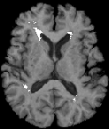
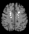
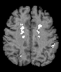
Figure 1. A representative axial section of a segmented training image. Figure 2. Two representative axial sections showing the results of manual segmentation of white-matter lesions (a, c) and the method described in this section (b, d).


Figure 1 shows a segmented normal training image. Figure 2 shows the results of segmentation, compared to segmentation performed manually by a neuroradiologist; note that there is good agreement between the computer-based method and the radiologist, except for a few small, false-positive regions near sulci.

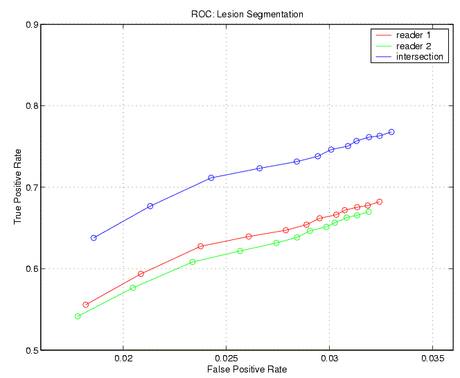
Figure 3. ROC curves for the white-matter-lesion segmentation algorithm, compared to two neuroradiologists and their intersection (regions of agreement).


Figure 3 shows receiver-operator characteristic (ROC) curves for two neuroradiologists, and for the intersection of their readings; in general, false-positive rates are low, even for high true-positive rates; however, there remain problems characterizing lesions near sulci, accounting for the true-positive rate that approaches 0.8.